Deep Learning for Expressive Piano Performances
Preface
For the last four years, a small team at Popgun has been studying the application of deep learning to music analysis and generation. This research has culminated in the release of Splash Pro - a free, AI-powered plugin for Digital Audio Workstations (DAWs). With the release of this blog, we hope to provide an accessible introduction to deep learning with music, by explaining some core projects we have worked on.
Introduction
In this post I want to describe the design of a model for expressive piano synthesis. The model, which we call ‘BeatNet’, is capable of analysing a piano performance and generating new pieces that imitate the original playing style. Before I get into the technical workings, here are a few samples generated by BeatNet:
In the style of “Yiruma - River Flows In You”
In the style of “Chopin - Nocturne in E-flat major, Op. 9, No. 2”
In the style of “Errol Garner - Misty”*
BeatNet is able to replicate many of the characteristics present in human piano performances, albeit with some weaknesses and limitations that I will address. To explain how this model works, I have split the remainder of the blog into two sections. Part I will discuss musical representations, while Part II will explore the model design and showcase more of its capabilities.
*Note: BeatNet does not model sustain pedal events. Sustain was manually added to this piece.
Part I - Representations of Music
In designing a model for music generation, it is critical to choose an appropriate representation. This choice determines which data can be faithfully encoded, the modelling techniques that are available, and the efficacy of the overall system. For this reason, I have decided to begin with a brief explanation of some common musical representations. If this all feels familiar to you, feel free to skip ahead to part II.
Audio
When we talk about audio in machine learning, we are typically referring to an array of time-domain samples. These samples are a digital approximation to the physical sound pressure wave. The quality of this approximation is determined by the sample rate and the bit-depth (see: PCM). In research, it is common to see sample rates of 16-22kHz. However, to capture the full range of human audible frequencies, most HiFi applications (e.g. music, podcasts, etc) use rates of around 44kHz (see: Nyquist Theorem).
Because of its high dimensionality, modelling raw audio is extremely challenging. For a generative model to reproduce audio structure on a timescale of a few seconds, it must capture the relationships between tens of thousands of samples. While it is becoming increasingly feasible to do this (see [1]), there are more efficient ways to encode piano performances.
Note: For an example of music modelling directly in the audio domain, see OpenAI’s Jukebox [2].
MIDI
MIDI is a technical standard allowing electronic instruments and computers to communicate. It comprises a sequence of ‘messages’, each describing a particular musical event or instruction. Instructions relating to the note timings, pitch and loudness (i.e. velocity) can be transmitted and stored. For example, a piano performance encoded as MIDI is a record of which notes were pressed, how forcefully and at what time.
To convert a MIDI file back into listenable audio, a piece of software replays these instructions and synthesizes the relevant notes. MIDI does not encode acoustic information, such as the instrument sound or the recording environment. For this reason it is drastically more efficient than audio, and it is a good starting point for our exploration.
When working with MIDI we use the terrific PrettyMIDI library by Colin Raffel. This abstracts away many complexities of the raw format. See Colin Raffel’s thesis for a more in-depth explanation of the MIDI file format.
Figure 1 - Für Elise in PrettyMIDI Format
Note(start=0.000000, end=0.305000, pitch=76, velocity=67)
Note(start=0.300000, end=0.605000, pitch=75, velocity=63)
Note(start=0.600000, end=0.905000, pitch=76, velocity=74)
Note(start=0.900000, end=1.205000, pitch=75, velocity=71)
...
Notice how succinctly we can represent Für Elise this way, and consider that the equivalent audio section contains approximately 50k samples (for a 44kHz recording).
Piano Roll
This will look familiar to anyone who has used a Digital Audio Workstation (DAW) such as GarageBand or Ableton. The vertical axis denotes pitch, and the horizontal axis denotes time. The velocity of each note is encoded by its magnitude. As well as providing an intuitive way to visualize MIDI, piano roll has some interesting properties for machine learning.
For example, consider the effect of raising the song’s pitch by one semitone, or delaying its onset by a few seconds. These transpositions preserve the spatial structure of the piano roll. When designing a model we can exploit this property by applying 2D Convolutional Neural Networks (CNN). Early experiments at Popgun tried exactly this, as did this project using PixelCNN. However, there are some serious drawbacks to this approach.
Figure 2 - Für Elise in Piano Roll Format
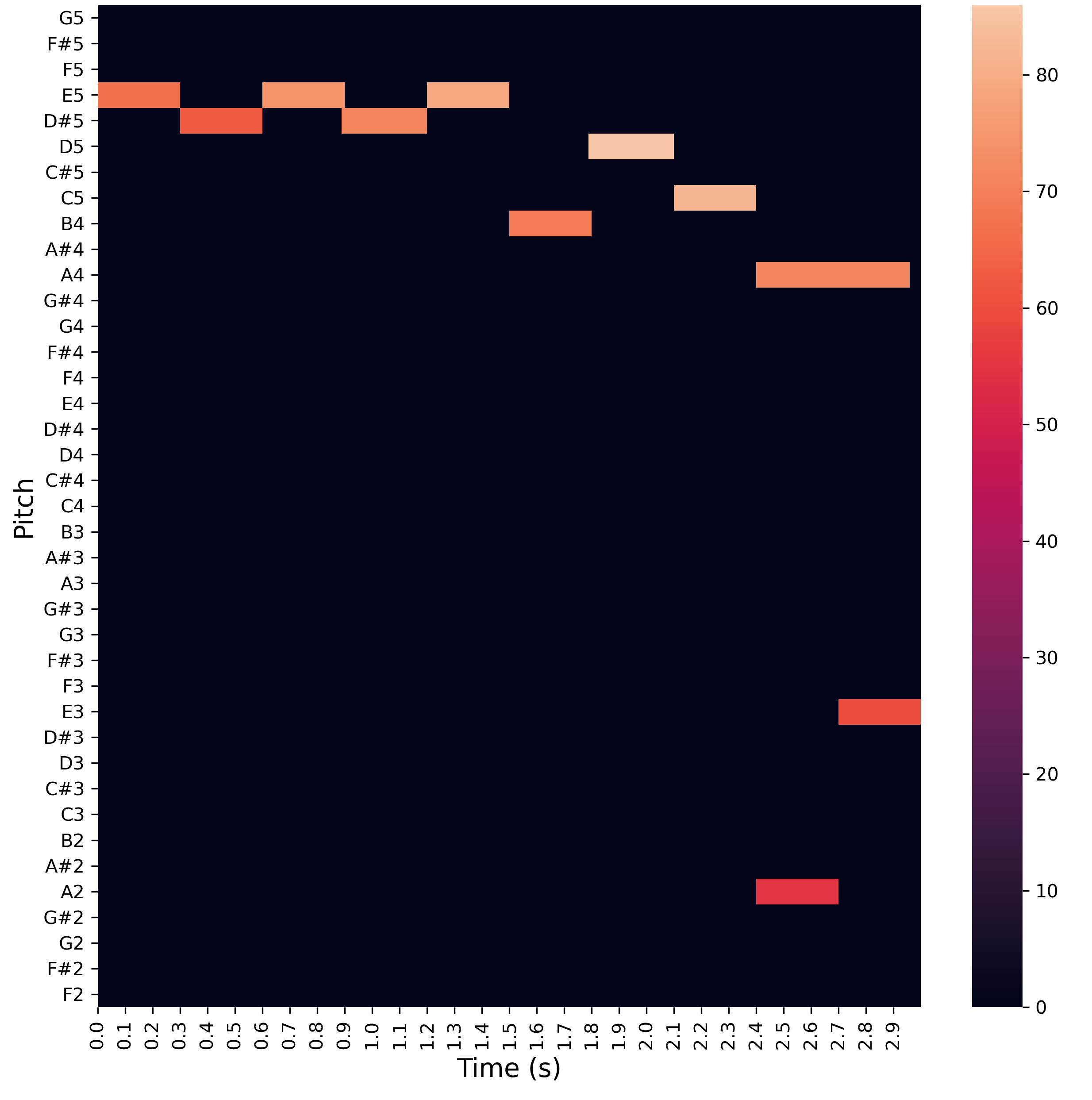
A typical song encoded as piano roll is incredibly sparse: nearly all entries are zero. Naively applying a CNN wastes a large amount of computation on entirely empty regions. It is also difficult to choose a suitable resolution for the time axis. If the original data is quantised, such that each note aligns perfectly with a uniform musical grid, we can choose the resolution based on the quantisation strength. However, this breaks down for expressive piano performances, where natural variations in timing are critical to the musicality.
Note: Many works have tried to model piano roll, using a broad range of neural net architectures. For those interested to learn more, this paper is a good starting point [16].
Time-Shift Format
In 2017 Google Magenta released a model called Performance RNN [3], which demonstrated the ability to model expressive piano performances with high fidelity. The key innovation was a new format that is highly suited to this task. For reasons that will become apparent, we refer to this “performance representation” simply as “time-shift”. Like MIDI, time-shift encodes music with a sequence of discrete musical events. What sets it apart is the unique way it encodes the progression of time. Instead of representing time along a specific axis (piano roll), or as a property of each individual note (MIDI), in time-shift there is a specific event that indicates the advancement of the piece.
Figure 3 - Für Elise in Time-Shift Format
272 - Set Velocity = 64
76  - Turn On MIDI Note 76 (E5)
317 - Advance Time by 0.3 Seconds
204 - Turn Off MIDI Note 76 (E5)
271 - Set Velocity = 60
75  - Turn On MIDI Note 75 (D#5)
317 - Advance Time by 0.3 Seconds
203 - Turn Off MIDI Note 75 (D#5)
274 - Set Velocity = 72
76  - Turn On MIDI Note 76 (E5)
317 - Advance Time by 0.3 Seconds
204 - Turn Off MIDI Note 76 (E5)
273 - Set Velocity = 68
75  - Turn On MIDI Note 75 (D#5)
317 - Advance Time by 0.3 Seconds
...
This one-dimensional sequence of tokens is similar to the encodings used in language models. This means that modern advances in NLP (e.g. ByteNet [4], Transformers [5]) can be readily applied to the time-shift format.
Figure 4 - An Explanation of the Time-Shift Events
0 - 127: Note on events
128 - 255: Note off events
256 - 287: 32 velocity change events
288 - 387: 100 quantized time-shift values (10ms -> 1000ms)
Note: We have not accounted for sustain pedal events, however it might be interesting to incorporate them in future work.
Part II - BeatNet: A Convolutional Model for Piano Music
In 2016, researchers at Google’s DeepMind lab released the now-famous WaveNet paper [1]. The core insight was that 1D convolutions could produce efficient sequence models, by eliminating the need for expensive recurrent computations during training. The efficacy was proven with a demo of raw audio generation. The publication of ByteNet [4] shortly afterwards, extended this idea to the domain of natural language processing.
Inspired by this work, Popgun developed its own ByteNet model for symbolic piano music. We refer to this work as “BeatNet”. The choice to use ByteNet over traditionally dominant RNNs was motivated by a few factors:
- The ability to capture long-term dependencies over hundreds or thousands of tokens
- Fast training
- Hype. WaveNet and ByteNet were the first papers to threaten the dominance of RNNs, before Transformer based architectures [5] exploded in popularity.
Data Collection and Processing
We curated a MIDI dataset by drawing from a number of online sources. One key source was the Yamaha e-Piano Competition Dataset, consisting of jazz and classical music performances. Another source was the Lakh MIDI Dataset, which contains a broader range of genres, including many contemporary pieces.
To create a model which generates highly expressive performances, we processed the data to filter out ‘low quality’ items. Anyone who has worked with MIDI datasets will appreciate that many songs sound ‘bad’. This raises some difficult problems: What is musical quality? How can we account for subjective preferences? Are some songs so weird we can confidently deem them ‘not musical’? Suffice to say, these problems are beyond the scope of this post.
Ultimately, our working solution can be summarised as this: An engineer listened to some data items, in each case proclaiming “Yep, this sounds musical” or “Nope, I don’t like it”. In the process, they developed automated heuristics to filter unwanted items, biasing the dataset towards songs that are subjectively ‘musical’. In the future it would be interesting to crowd-source these assessments, or to devise heuristics based on music theory instead.
A Working Prototype
We completed our first working prototype in July 2017. It is essentially an unconditional ByteNet [4] decoder, operating over time-shift format sequences. Figure 5 illustrates the basic generation procedure.
Figure 5 - Schematic of BeatNet Generation
At each step, BeatNet outputs a probability distribution over the next time-shift token, based on the historical context. To generate a song, we prime the model with a sequence from the held-out test set, and sample a predicted continuation. Here is a sample from this model:
An Early Sample From BeatNet
Notice the presence of natural variations in timing and loudness, mimicking the kinds of features present in a human performance. Despite some interesting flourishes, the model tends to wander aimlessly, with limited evidence of planning or long term structure. The timing is also unusual, since the model has no concept of time signatures or rhythms.
For user-facing applications, this kind of ‘unconditional’ model has very limited control; only the priming sequence (and a few minor generation settings) can be adjusted. One way to improve this is to introduce a latent variable.
Improving Control with Latent Variables
Variational Autoencoders (VAEs) [6] are a popular generative modelling technique, with applications in an increasing number of domains, such as images [7], molecule synthesis [8], symbolic music [9][10] and speech synthesis [11]. A lot has been written about VAEs by other authors [12][13][14], so I will not give a comprehensive explanation here. What’s important is this: VAEs provide a principled way to learn the unspecified factors of variation in a dataset. To illustrate why this is useful, consider two pathways to control in our piano model:
-
The desired model controls (e.g. “loudness”, “tempo”, “key”) are specified in advance. For each dataset item (or a large subset) we collect labels corresponding to these controls. We provide these labels as an additional input to the model during training. When generating a new song these features can be manipulated to steer the output.
-
A VAE is trained to automatically discover the latent factors of variation in the data. After training, a musically trained listener explores these factors (e.g. by interpolating on each dimension) and observes the effect on the model output. Based on this exploration, we devise a post-hoc interpretation of each latent dimension. By exposing these features to the user they can steer the model as per (1).
There are trade-offs between these approaches. If the desired control features can be readily extracted for each data item then (1) becomes feasible. However, in our experiments we observed that features defined this way tend to have natural correlations in the dataset. This can negatively impact the output quality if the user defines an implausible configuration at generation time. Contrast this with the approach in (2), whereby the VAE objective encourages independence of the learned control features.
Furthermore, consider that we might like to control certain abstract features, such as ‘style’ or ‘genre’, which are difficult to formally define. The VAE sidesteps this issue, by simply learning features that explain the variability in the data. It is possible that a certain latent dimension or subspace will map to human notions of ‘genre’ or ‘style’, but there are no guarantees; it can be difficult to interpret the learned features. In practice, we make two observations:
-
It is often possible to find an interpretable subset of latent dimensions to expose as user controls.
-
Irrespective of 1., a latent space provides novel mechanisms for user control, such as musical interpolation and style transfer.
BeatNet VAE
In BeatNet VAE we introduce a sequence of latent variables to help guide the model generation. The architecture is very similar to Google Magenta’s NSynth [15]. A convolutional encoder embeds the input into a compressed latent representation, which is then provided as additional context to the ByteNet decoder. The VAE objective encourages these vectors to follow a simple distribution (i.e. standard normal), and provides a penalty on the amount of information they can contain. By tuning the size of the latent vectors and the regularisation term, it is possible to learn a representation that explains some (but importantly not all) of the variation in the sequence. By holding this latent variable constant, we can sample many diverse outputs which inherit the ‘style’ of a given input.
A Continuation of Für Elise with Beatnet VAE
Für Elise MIDI sourced from 8notes with permission.
This snippet demonstrates how BeatNet VAE can generate continuations of given input sequence. The input runs for 18s, with the model response following. Latent variables derived from the original piece help to guide the continuation, transferring qualities such as the dynamics, key and playing style. Note that compared with the unconditional model, BeatNet VAE does a much better job of playing consistently.
Figure 6 - Event Probabilities for Für Elise Continuation
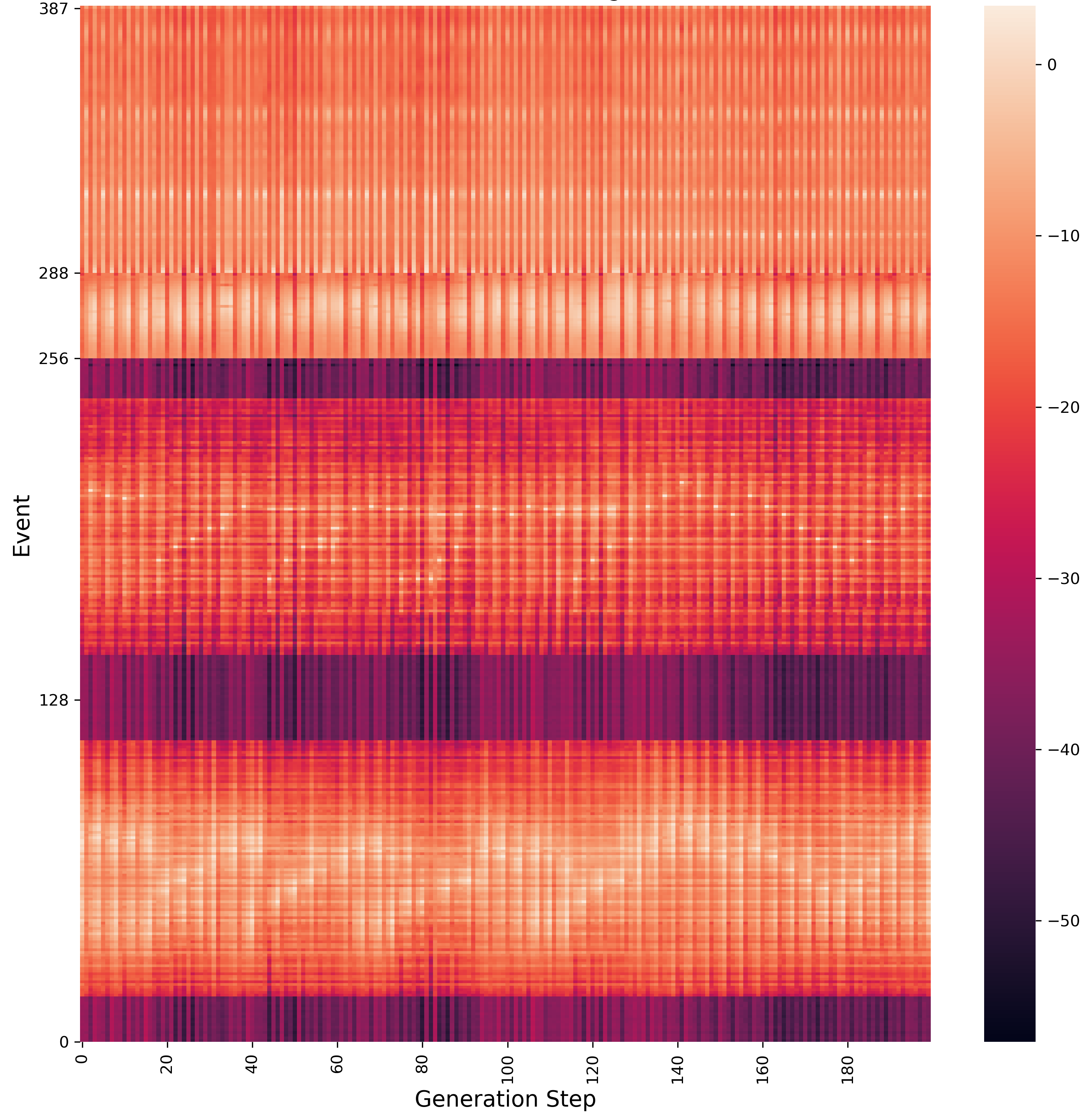
Figure 6 shows the probability BeatNet assigns to each token during the first 200 steps of generation. The y-axis tracks the different event types, starting with ‘note on’ events From y=0 to y=127. ‘Note off’ events are above that, and so on according to the time-shift specification. The dark horizontal bands correspond to notes that are outside the range of piano music in the training data.
Figure 7 - Probabilities for ‘Note On’ Events
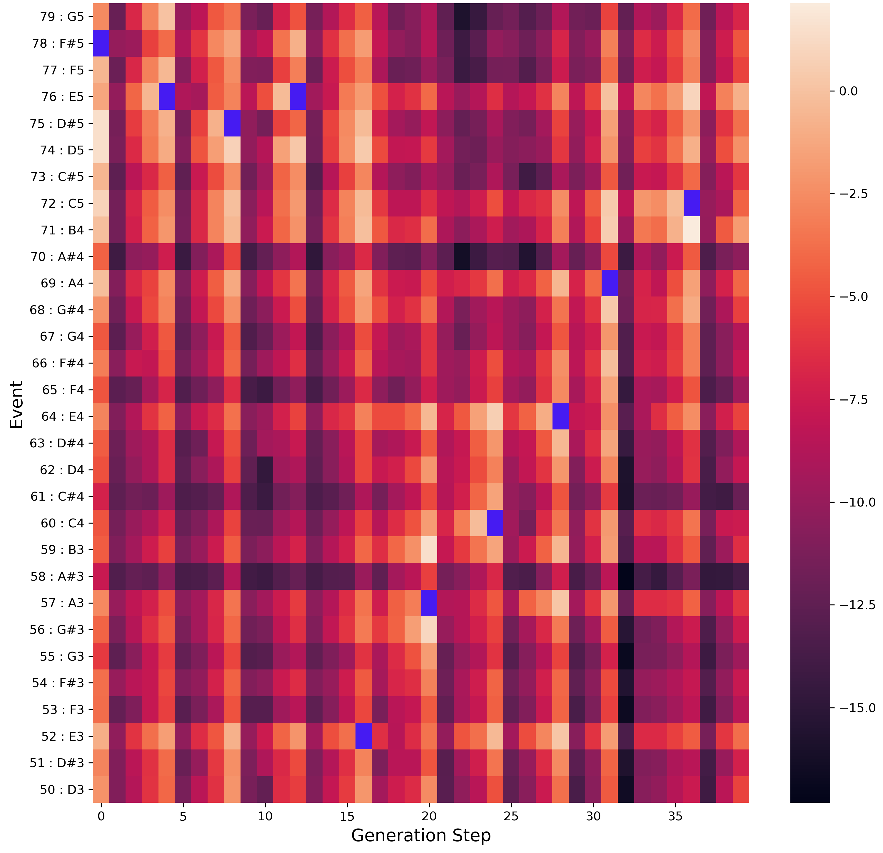
Figure 7 gives a zoomed-in picture of the same probabilities. We are focusing on the ‘note on’ events for the first 40 generation steps. Figure 8 (below) presents the same phrase as piano roll for comparison. The tokens selected by BeatNet at each step have been highlighted in purple (remember that only ‘note on’ tokens are shown).
To understand what’s going on lets consider one column in isolation. At x=20 BeatNet elects to play the note
A3 (token 57). Given that we are in A-minor it seems reasonable that BeatNet has assigned a high probability to
B3 (a diatonic note), and a low probability to the A#3 (a dissonant minor 2nd). At each step a multitude of
branching trajectories are possible, though some are much more likely than others.
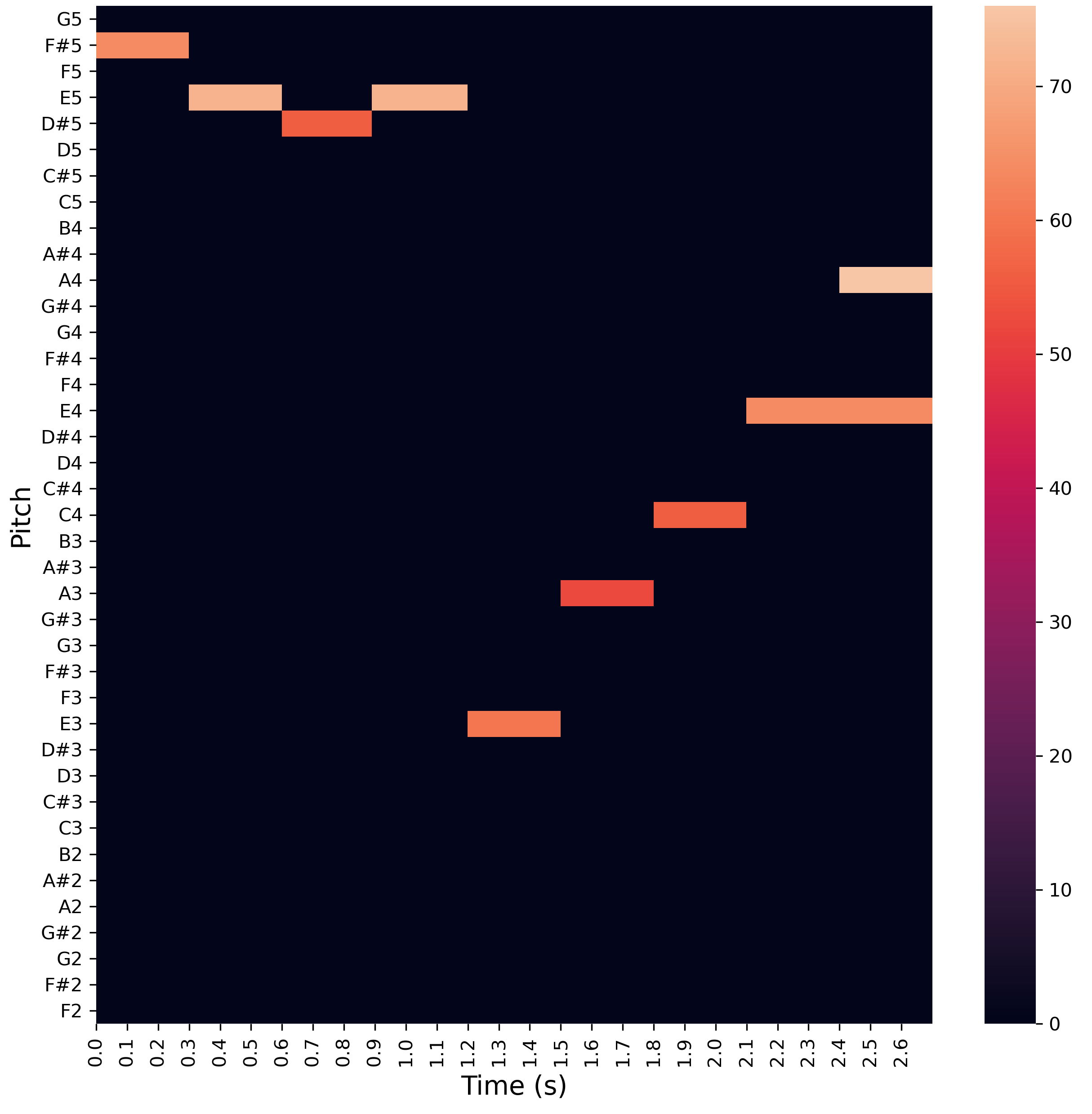
Figure 8 - Für Elise Continuation in Piano Roll Format.
Further Reading
For more applications of machine learning to creative tasks, the Google Magenta blog contains many interesting projects.
Special Thanks
This project was a joint effort from the Popgun team. I would like to especially thank Adam Hibble for leading the team during this project. If you have any technical questions feel free to reach out on twitter. For other inquiries email info@popgun.ai .